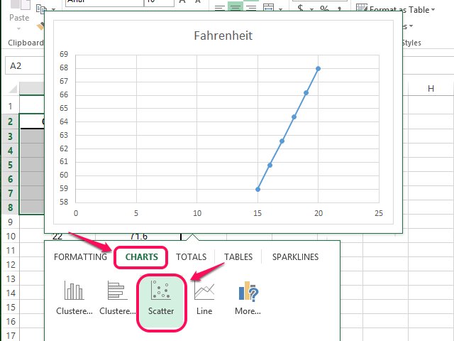
42 excel scatter diagram with labels

Labeling points in excel scatter diagram - YouTube Showing how to put labels on points of an excel scatter diagram. The video can help familiarize with plotting a scatter diagram, putting trendlines, formatting the chart, x and y axis, use of... How to use a macro to add labels to data points in an xy scatter chart ... In Microsoft Office Excel 2007, follow these steps: Click the Insert tab, click Scatter in the Charts group, and then select a type. On the Design tab, click Move Chart in the Location group, click New sheet , and then click OK. Press ALT+F11 to start the Visual Basic Editor. On the Insert menu, click Module.

How to create a scatter plot and customize data labels in Excel During Consulting Projects you will want to use a scatter plot to show potential options. Customizing data labels is not easy so today I will show you how th...

Excel scatter diagram with labels

Excel 2019/365: Scatter Plot with Labels - YouTube How to add labels to the points on a scatter plot. Find, label and highlight a certain data point in Excel scatter … 10.10.2018 · As the result, you will have a scatter plot with the average point labeled and highlighted: That's how you can spot and highlight a certain data point on a scatter diagram. To have a closer look at our examples, you are welcome to download our sample Excel Scatter Plot workbook. I thank you for reading and hope to see you on our blog next week. Add a trend or moving average line to a chart On an unstacked, 2-D, area, bar, column, line, stock, xy (scatter), or bubble chart, click the data series to which you want to add a trendline or moving average, or do the following to select the data series from a list of chart elements: Click anywhere in the chart. This displays the Chart Tools, adding the Design, Layout, and Format tabs.

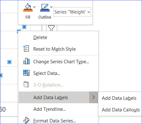
Excel scatter diagram with labels. How to Add Labels to Scatterplot Points in Excel - Statology Step 3: Add Labels to Points. Next, click anywhere on the chart until a green plus (+) sign appears in the top right corner. Then click Data Labels, then click More Options…. In the Format Data Labels window that appears on the right of the screen, uncheck the box next to Y Value and check the box next to Value From Cells. Improve your X Y Scatter Chart with custom data labels Select the x y scatter chart. Press Alt+F8 to view a list of macros available. Select "AddDataLabels". Press with left mouse button on "Run" button. Select the custom data labels you want to assign to your chart. Make sure you select as many cells as there are data points in your chart. Press with left mouse button on OK button. Back to top How to Create a Quadrant Chart in Excel – Automate Excel We’re almost done. It’s time to add the data labels to the chart. Right-click any data marker (any dot) and click “Add Data Labels.” Step #10: Replace the default data labels with custom ones. Link the dots on the chart to the corresponding marketing channel names. To do that, right-click on any label and select “Format Data Labels.” XY Scatter Diagram - Excel Help Forum I saw your axis labels are Y = Consequence and X = Prob but the data source for the chart in your file is Y = Prob and X = Consq, so I changed it in this attached file to be align with axis title. Attached Files Analysis.xlsx‎ (60.2 KB, 6 views) Download Register To Reply 03-21-2022, 12:40 PM #3 MarvinP Forum Guru Join Date 07-23-2010 Location

Scatter Diagram Help - BPI Consulting If you do, the program will add these as the labels for the X axis and Y axis. 2. Select "Scatter" from the "Cause and Effect" panel on the SPC for Excel ribbon. 3. The input screen for the scatter diagram is displayed. The program sets the initial X and Y ranges as the range that is selected on the worksheet. How to Find and Use Excel's Free Flowchart Templates - Lifewire 15.12.2020 · Use the SmartArt templates to create a flowchart in an Excel worksheet. Updated to include Excel 2019. G A S REGULAR. Menu. Lifewire. Tech for Humans . Best Products Audio Camera & Video Car Audio & Accessories Computers & Laptops Computer Accessories Game Consoles Gifts Networking Phones Smart Home Software Tablets Toys & Games TVs … How to Create a Sankey Diagram in Excel Spreadsheet Components of a Sankey Diagram in Excel. A Sankey is a minimalist diagram that consists of the following: Nodes: This is an element linked by “Flows.” Furthermore, it represents the events in each path. Flows: Flows link the nodes. And each flow is specified by the names of its source and target nodes in the “from” and “to” fields ... excel - How to label scatterplot points by name? - Stack Overflow select a label. When you first select, all labels for the series should get a box around them like the graph above. Select the individual label you are interested in editing. Only the label you have selected should have a box around it like the graph below. On the right hand side, as shown below, Select "TEXT OPTIONS".

Available chart types in Office - support.microsoft.com When you create a chart in an Excel worksheet, a Word document, or a PowerPoint presentation, you have a lot of options. Whether you’ll use a chart that’s recommended for your data, one that you’ll pick from the list of all charts, or one from our selection of chart templates, it might help to know a little more about each type of chart.. Click here to start creating a chart. Excel Scatter Chart with Labels - Super User Move the button down and out of the way of your data if you have more than a few columns. Paste your data in on top of the film data. Create scatter plots by selecting two column at a time and insert scatter (plot). Clicking on the button, which will add labels. Easy. How To Create Scatter Chart in Excel? - EDUCBA To apply the scatter chart by using the above figure, follow the below-mentioned steps as follows. Step 1 - First, select the X and Y columns as shown below. Step 2 - Go to the Insert menu and select the Scatter Chart. Step 3 - Click on the down arrow so that we will get the list of scatter chart list which is shown below. Scatter Graph - Overlapping Data Labels - Excel Help Forum We are not able to work with or manipulate a picture of one and nobody wants to have to recreate your data from scratch. 1. Make sure that your sample data are REPRESENTATIVE of your real data. The use of unrepresentative data is very frustrating and can lead to long delays in reaching a solution. 2.

How to Make an XY Graph on Excel | Techwalla.com

EOF

How to Make a Scatter Chart - ExcelNotes

How to display text labels in the X-axis of scatter chart in Excel? Display text labels in X-axis of scatter chart Actually, there is no way that can display text labels in the X-axis of scatter chart in Excel, but we can create a line chart and make it look like a scatter chart. 1. Select the data you use, and click Insert > Insert Line & Area Chart > Line with Markers to select a line chart. See screenshot: 2.

How to Create a Scatter Diagram in Excel - YouTube

How to plot a ternary diagram in Excel - Chemostratigraphy.com 13.02.2022 · Insert a Scatter Chart (XY diagram), e.g., ‘Scatter with Straight Lines’ (Figure 9) using the XY coordinates for the triangle from columns AA and AB. To make it into an equilateral triangle resize the chart area accordingly; for example 10 columns wide and 30 rows high, as in Figure 10. (You can check by drawing a triangle (Insert > Shapes > Triangle); hold the Shift …

Scatter Chart in Microsoft Excel

Add Custom Labels to x-y Scatter plot in Excel Step 1: Select the Data, INSERT -> Recommended Charts -> Scatter chart (3 rd chart will be scatter chart) Let the plotted scatter chart be. Step 2: Click the + symbol and add data labels by clicking it as shown below. Step 3: Now we need to add the flavor names to the label. Now right click on the label and click format data labels.

Line Chart in Excel - Easy Excel Tutorial

How to Create Venn Diagram in Excel – Free Template Download First, let’s add data labels. Right-click on the data marker representing Series “Pepsi” and choose “Add Data Labels.” Step #15: Customize data labels. Replace the default values with the custom labels you previously designed. Right-click on any data label and choose “Format Data Labels.” Once the task pane pops up, do the following: