40 excel pivot table labels
How to rename group or row labels in Excel PivotTable? You can rename a group name in PivotTable as to retype a cell content in Excel. Click at the Group name, then go to the formula bar, type the new name for the group. Rename Row Labels name To rename Row Labels, you need to go to the Active Field textbox. 1. Click at the PivotTable, then click Analyze tab and go to the Active Field textbox. 2. Turn Repeating Item Labels On and Off - Excel Pivot Tables To change the setting: Right-click one of the items in the field - in this example I'll right-click on "Cookies". In the pop-up menu, click Field Settings. In the Field Settings window, click the Layout & Print tab. Add a check mark to Repeat Item Labels, and click OK. Now, the Category names appear in each row.
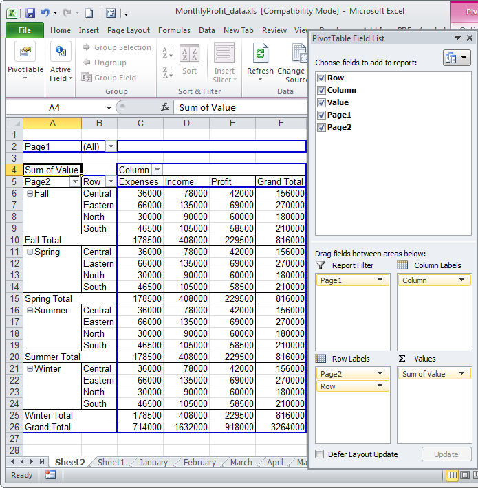
Excel 2016 Pivot table Row and Column Labels - Microsoft Community In Excel 2016 I've found when I create a pivot table it unhelpfully shows 'Row Labels' and 'Column Labels' instead of my field names, although in the top left cell it says 'Count of' and then inserts the correct field name. Years ago when I last used Excel it automatically put the field names in all three heading cells.
Excel pivot table labels
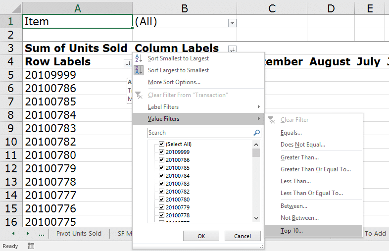
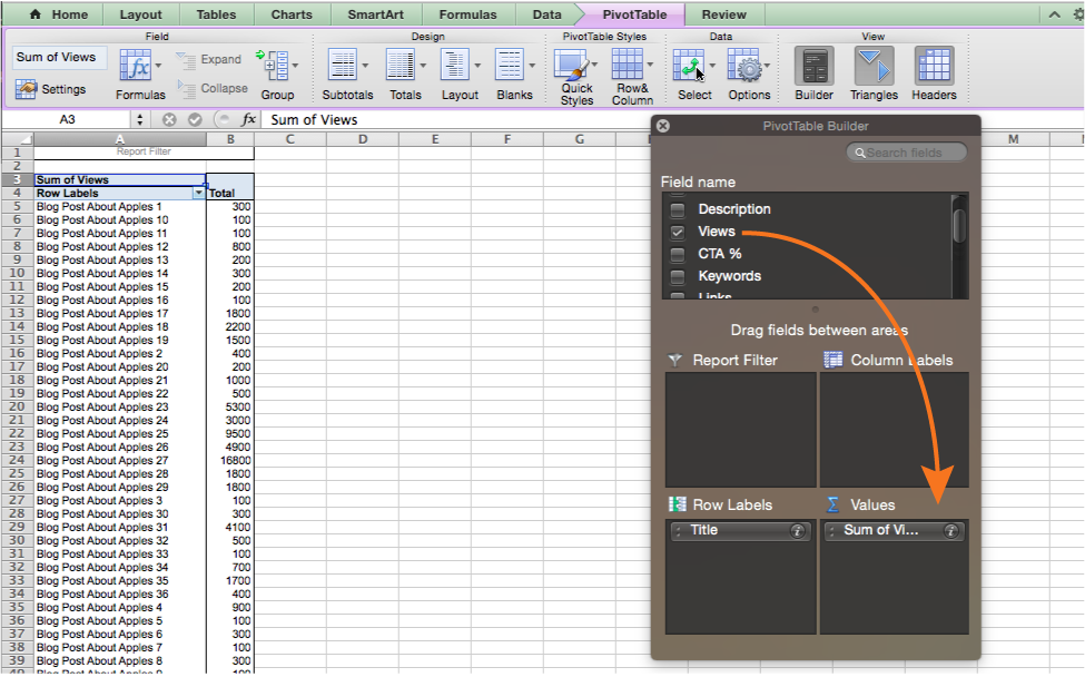
Data Labels in Excel Pivot Chart (Detailed Analysis) 7 Suitable Examples with Data Labels in Excel Pivot Chart Considering All Factors 1. Adding Data Labels in Pivot Chart 2. Set Cell Values as Data Labels 3. Showing Percentages as Data Labels 4. Changing Appearance of Pivot Chart Labels 5. Changing Background of Data Labels 6. Dynamic Pivot Chart Data Labels with Slicers 7. Pivot table row labels side by side - Excel Tutorials You can copy the following table and paste it into your worksheet as Match Destination Formatting. Now, let's create a pivot table ( Insert >> Tables >> Pivot Table) and check all the values in Pivot Table Fields. Fields should look like this. Right-click inside a pivot table and choose PivotTable Options…. Check data as shown on the image below. How to Customize Your Excel Pivot Chart Data Labels The Data Labels command on the Design tab's Add Chart Element menu in Excel allows you to label data markers with values from your pivot table. When you click the command button, Excel displays a menu with commands corresponding to locations for the data labels: None, Center, Left, Right, Above, and Below.
Excel pivot table labels. excel - Custom column labels in PivotTable - Stack Overflow Select the data from which the pivot table is from. highlight the column in which the "b" is in. find and replace all the "b" with "In Progress". Update the Pivot table. OR. Copy the data from the pivot table and Paste it as text delimited I believe. -Change the "b" to "In Progress". Please respond if it isnt clear so I can go into further detail. Pivot Table "Row Labels" Header Frustration - Microsoft Tech Community Pivot Table "Row Labels" Header Frustration. Hi Everyone please help I can't change my headers from Row Labels in a Pivot Table. Using Excel 365. Labels: Pivot Table Row Labels - Microsoft Community If you go to PivotTable Tools > Analyze > Layout > Report Layout > Show in Tabular Form, your column headers will be used for the row labels. Every once in a while there's a sudden gust of gravity... Report abuse 1 person found this reply helpful · Was this reply helpful? Yes No A. User Replied on December 19, 2017 Move Row Labels in Pivot Table - Excel Pivot Tables When you add fields to the row labels area in a pivot table, the field's items are automatically sorted. See how you can manually move those labels, to put them in a different order. There's a video and written steps below. In the screen shot below, the districts are listed alphabetically, from Central to West.
Use column labels from an Excel table as the rows in a Pivot Table Highlight your current table, including the headers Then from the Data section of the ribbon, select From Table Highlight all the columns containing data, but not the Year column, and then select Unpivot Columns Close the dialog and keep the changes. Excel should place the unpivoted data into a new worksheet, looking something like this: How to Select Parts of Excel Pivot Table - Contextures Select Labels in a Pivot Table — Select Labels in Pivot Table · Point to the top border of a Row Label heading · When the pointer changes to a thick ... How to Move Excel Pivot Table Labels Quick Tricks To move a pivot table label to a different position in the list, you can use commands in the right-click menu: Right-click on the label that you want to move Click the Move command Click one of the Move subcommands, such as Move [item name] Up The existing labels shift down, and the moved label takes its new position. Type Over Another Label Design the layout and format of a PivotTable In the PivotTable Options dialog box, click the Layout & Format tab, and then under Layout, select or clear the Merge and center cells with labels check box. Note: You cannot use the Merge Cells check box under the Alignment tab in a PivotTable. Change the display of blank cells, blank lines, and errors
Automatic Row And Column Pivot Table Labels - How To Excel At Excel Select the data set you want to use for your table The first thing to do is put your cursor somewhere in your data list Select the Insert Tab Hit Pivot Table icon Next select Pivot Table option Select a table or range option Select to put your Table on a New Worksheet or on the current one, for this tutorial select the first option Click Ok Labels · MarionCoutarel/update_excel_pivot_table · GitHub Creating series of Excel files with pivot tables updating data in template Excel files and refreshing pivot table - Labels · MarionCoutarel/update_excel_pivot_table Pivot table row labels in separate columns • AuditExcel.co.za Our preference is rather that the pivot tables are shown in tabular form (all columns separated and next to each other). You can do this by changing the report format. So when you click in the Pivot Table and click on the DESIGN tab one of the options is the Report Layout. Click on this and change it to Tabular form. How to make row labels on same line in pivot table? Make row labels on same line with PivotTable Options You can also go to the PivotTable Options dialog box to set an option to finish this operation. 1. Click any one cell in the pivot table, and right click to choose PivotTable Options, see screenshot: 2.
Frequency Distribution in Excel - Easy Excel Tutorial
get a row label from pivot table - Microsoft Tech Community Creating PivotTable add data to data model by checking Create PivotTable and after that convert it to cube formulas. Now you may take these formulas and convert it to form you need, for example in H3 it could be =CUBEVALUE( "ThisWorkbookDataModel", CUBEMEMBER("ThisWorkbookDataModel", " [Measures].
How to Format Excel PivotTables for Even Greater Effect - K2E Canada Inc
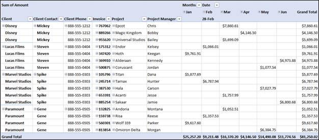
How to add column labels in pivot table [SOLVED] Steps:-. Click any date in the Column Lables. Click Pivot table options tab on the Ribbon. In the Options Table, Click Group Field option. Click Months then click Ok. Thats it. check the attached file:-. Attached Files. PIVOT.xlsx (30.3 KB, 6 views) Download.

Excel pivot filters: Charts
How to Use Excel Pivot Table Label Filters Right-click a cell in the pivot table, and click PivotTable Options. In the PivotTable Options dialog box, click the Totals & Filters tab In the Filters section, add a check mark to 'Allow multiple filters per field.' Click the OK button, to apply the setting and close the dialog box. Quick Way to Hide or Show Pivot Items

33 Pivot Table Blank Row Label - Labels Database 2020
Pivot Table Row Labels In the Same Line - Beat Excel! It is a common issue for users to place multiple pivot table row labels in the same line. You may need to summarize data in multiple levels of detail while rows labels are side by side. In this post I'm going to show you how to do it. ... After creating a pivot table in Excel, you will see the row labels are listed in only one column. But, if ...

Creating Pivot Tables in Excel for Exported Data – Teaching & Learning
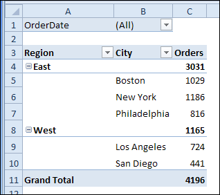
How to Use Label Filters for Text in the Pivot Table? - MS Excel ... Label Filters for Text in the Pivot Table - A Glance: You can use Row Label Filter or Column Label Filter in the pivot table to filter your required data based on the field items. If you have a huge list of data and you want to filter it based on the text string, then you can use this filter to make your work much easier.
Repeat Pivot Table Labels in Excel 2010 - Excel Pivot TablesExcel Pivot Tables
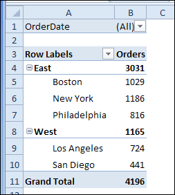
Excel: How to Sort Pivot Table by Date - Statology Often you may want to sort the rows in a pivot table in Excel by date. Fortunately this is easy to do using the sorting options in the dropdown menu within the Row Labels column of a pivot table. The following example shows exactly how to do so. Example: Sort Pivot Table by Date in Excel
34 Excel Pivot Table Label Filter Contains Multiple Values - Labels Design Ideas 2020
How To Create A Ms Excel Pivot Table An Introduction Simple Tax India Read Or Download Gallery of how to create a ms excel pivot table an introduction simple tax india - Pivot Table Row Labels | how to create a pivot table with multiple columns and rows cabinets, move row labels in pivot table excel pivot tables, pivot table multiple row labels side by side, get a row label from pivot table microsoft tech community,
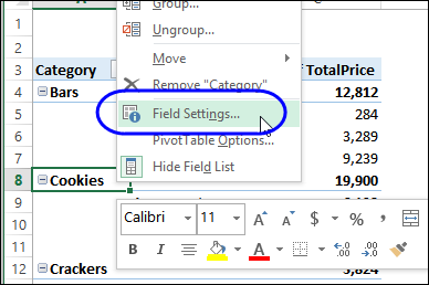
Turn Repeating Item Labels On and Off – Excel Pivot Tables
Repeat All Item Labels In An Excel Pivot Table | MyExcelOnline You can then select to Repeat All Item Labels which will fill in any gaps and allow you to take the data of the Pivot Table to a new location for further analysis. STEP 1: Click in the Pivot Table and choose PivotTable Tools > Options (Excel 2010) or Design (Excel 2013 & 2016) > Report Layouts > Show in Outline/Tabular Form
![[5 Steps] How To Make Ranking Charts With Excel Pivot Tables - Moz](https://d1avok0lzls2w.cloudfront.net/img_uploads/column-labels.png)
[5 Steps] How To Make Ranking Charts With Excel Pivot Tables - Moz
Repeat item labels in a PivotTable - support.microsoft.com Right-click the row or column label you want to repeat, and click Field Settings. Click the Layout & Print tab, and check the Repeat item labels box. Make sure Show item labels in tabular form is selected. Notes: When you edit any of the repeated labels, the changes you make are applied to all other cells with the same label.
Group data in an Excel Pivot Table
How to reset a custom pivot table row label Now go back to your Pivot and refresh it to find the Problem column and the duplicate column you just made. 5. Enter both fields into the pivot table and you will see the duplicate column has the original values while the Problem column maintains the problem labels. Monday, April 27, 2015 8:39 AM 0 Sign in to vote

How Do Pivot Tables Work? - Excel Campus | Pivot table, Row labels, Excel
How to Group Rows in Excel Pivot Table (3 Ways) - ExcelDemy Now select any number in the Row Labels of the table. Then right-click and select Group as shown below. Then, enter the Starting ( 60) and Ending ( 100) numbers and the difference ( 10) by which you want to group them. Next, hit OK. Finally, you will see the numbers grouped together as shown in the picture below.👇.
Repeat Pivot Table Labels in Excel 2010 – Excel Pivot Tables
How to Customize Your Excel Pivot Chart Data Labels The Data Labels command on the Design tab's Add Chart Element menu in Excel allows you to label data markers with values from your pivot table. When you click the command button, Excel displays a menu with commands corresponding to locations for the data labels: None, Center, Left, Right, Above, and Below.

Filtering Grand Total Amounts Within Excel Pivot Tables | AccountingWEB
Pivot table row labels side by side - Excel Tutorials You can copy the following table and paste it into your worksheet as Match Destination Formatting. Now, let's create a pivot table ( Insert >> Tables >> Pivot Table) and check all the values in Pivot Table Fields. Fields should look like this. Right-click inside a pivot table and choose PivotTable Options…. Check data as shown on the image below.

Excel Pivot Table Report - Sort Data in Row & Column Labels & in Values Area, use Custom Lists
Data Labels in Excel Pivot Chart (Detailed Analysis) 7 Suitable Examples with Data Labels in Excel Pivot Chart Considering All Factors 1. Adding Data Labels in Pivot Chart 2. Set Cell Values as Data Labels 3. Showing Percentages as Data Labels 4. Changing Appearance of Pivot Chart Labels 5. Changing Background of Data Labels 6. Dynamic Pivot Chart Data Labels with Slicers 7.

Excel Pivot Table Report - Sort Data in Row & Column Labels & in Values Area, use Custom Lists

Choosing PivotTable Layouts | Microsoft Excel - Pivot Tables

Excel Pivot Table Report - Sort Data in Row & Column Labels & in Values Area, use Custom Lists
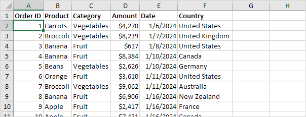
How to Create a Pivot Table in Excel: A Step-by-Step Tutorial (With Video)
Post a Comment for "40 excel pivot table labels"